mapreduce.py

#

On day 4, we saw how to process text data using the Enron email dataset. In reality, we only processed a small fraction of the entire dataset: about 15 megabytes of Kenneth Lay's emails. The entire dataset containing many Enron employees' mailboxes is 1.3 gigabytes, about 87 times than what we worked with. And what if we worked on GMail, Yahoo! Mail, or Hotmail? We'd have several petabytes worth of emails, at least 71 million times the size of the data we dealt with.

All that data would take a while to process, and it certainly couldn't fit on or be crunched by a single laptop. We'd have to store the data on many machines, and we'd have to process it (tokenize it, calculate tf-idf) using multiple machines. There are many ways to do this, but one of the more popular recent methods of parallelizing data computation is based on a programming framework called MapReduce, an idea that Google presented to the world in 2004. Luckily, you do not have to work at Google to benefit from MapReduce: an open-source implementation called Hadoop is available for your use!

You might worry that we don't have hundreds of machines sitting around for us to use them. Actually, we do! Amazon Web Services offers a service called Elastic MapReduce (EMR) that gives us access to as many machines as we would like for about 10 cents per hour of machine we use. Use 100 machines for 2 hours? Pay Amazon aroud $2.00. If you've ever heard the buzzword cloud computing, this elastic service is part of the hype.

Let's start with a simple word count example, then rewrite it in MapReduce, then run MapReduce on 20 machines using Amazon's EMR, and finally write a big-person MapReduce workflow to calculate TF-IDF!

Setup

We're going to be using two files, dataiap/day5/term_tools.py and dataiap/day5/package.tar.gz. Either write your code in the dataiap/day5 directory, or copy these files to the directory where your work lives.

Counting Words

We're going to start with a simple example that should be familiar to you from day 4's lecture. First, unzip the JSON-encoded Kenneth Lay email file:

unzip dataiap/datasets/emails/kenneth_json.zip
#

This will result in a new file called lay-k.json, which is JSON-encoded. What is JSON? You can think of it like a text representation of python dictionaries and lists. If you open up the file, you will see on each line something that looks like this:

{"sender": "rosalee.fleming@enron.com", "recipients": ["lizard_ar@yahoo.com"], "cc": [], "text": "Liz, I don't know how the address shows up when sent, but they tell us it's \nkenneth.lay@enron.com.\n\nTalk to you soon, I hope.\n\nRosie", "mid": "32285792.1075840285818.JavaMail.evans@thyme", "fpath": "enron_mail_20110402/maildir/lay-k/_sent/108.", "bcc": [], "to": ["lizard_ar@yahoo.com"], "replyto": null, "ctype": "text/plain; charset=us-ascii", "fname": "108.", "date": "2000-08-10 03:27:00-07:00", "folder": "_sent", "subject": "KLL's e-mail address"}

It's a dictionary representing an email found in Kenneth Lay's mailbox. It contains the same content that we dealt with on day 4, but encoded into JSON, and rather than one file per email, we have a single file with one email per line.

Why did we do this? Big data crunching systems like Hadoop don't deal well with lots of small files: they want to be able to send a large chunk of data to a machine and have to crunch on it for a while. So we've processed the data to be in this format: one big file, a bunch of emails line-by-line. If you're curious how we did this, check out dataiap/day5/emails_to_json.py.

Aside from that, processing the emails is pretty similar to what we did on day 4. Let's look at a script that counts the words in the text of each email (Remember: it would help if you wrote and ran your code in dataiap/day5/... today, since several modules like term_tools.py are available in that directory).

import sys
from collections import defaultdict
from mrjob.protocol import JSONValueProtocol
from term_tools import get_terms

input = open(sys.argv[1])
words = defaultdict(lambda: 0)
for line in input:
    email = JSONValueProtocol.read(line)[1]
    for term in get_terms(email['text']):
        words[term] += 1

for word, count in words.items():
    print word, count
#

You can save this script to exercise1.py and then run python exercise1.py dataiap/datasets/emails/lay-k.json. It will print the word count in due time. get_terms is similar to the word tokenizer we saw on day 4. words keeps track of the number of times we've seen each word. email = JSONValueProtocol.read(line)[1] uses a JSON decoder to convert each line into a dictionary called email, that we can then tokenize into individual terms.

As we said before, running this process on several petabytes of data is infeasible because a single machine might not have petabytes of storage, and we would want to enlist multiple computers in the counting process to save time.

We need a way to tell the system how to divide the input data amongst multiple machines, and then combine all of their work into a single count per term. That's where MapReduce comes in!

Motivating MapReduce

You may have noticed that the various programs we have written in previous exercises look somewhat repetitive.

Remember when we processed the campaign donations dataset to create a histogram? We basically:

  1. extracted the candidate name and donation amount from each line and computed the histogram bucket for the amount
  2. grouped the donations by candidate name and donation amount.
  3. summarized each (candidate, donation) bucket by counting the number of donations.

Now consider computing term frequency in the previous class. We:

  1. cleaned and extracted terms from each email file
  2. grouped the terms by which folder they were from
  3. summarized each folder's group by counting the number of times each term was seen.

This three-step pattern of 1) extracting and processing from each line or file, 2) grouping by some attribute(s), and 3) summarizing the contents of each group is common in data processing tasks. We implemented step 2 by adding elements to a global dictionary (e.g., folder_tf[e['folder']].update in day 4's code). We implemented step 3 by counting or summing the values in the dictionary.

Using a dictionary like this works because the dictionary fits in memory. However if we had processed a lot more data, the dictionary may not fit into memory, and it'll take forever to run. Then what do we do?

The researchers at Google also noticed this problem, and developed a framework called MapReduce to run these kinds of patterns on huge amounts of data. When you use this framework, you just need to write functions to perform each of the three steps, and the framework takes care of running the whole pattern on one machine or a thousand machines! They use a different terminology for the three steps:

  1. Map (from each)
  2. Shuffle (grouping by)
  3. Reduce (summarize)

OK, now that you've seen the motivation behind the MapReduce technique, let's actually try it out.

MapReduce

Say we have a JSON-encoded file with emails (3,000,000 emails on 3,000,000 lines), and we have 3 computers to compute the number of times each word appears.

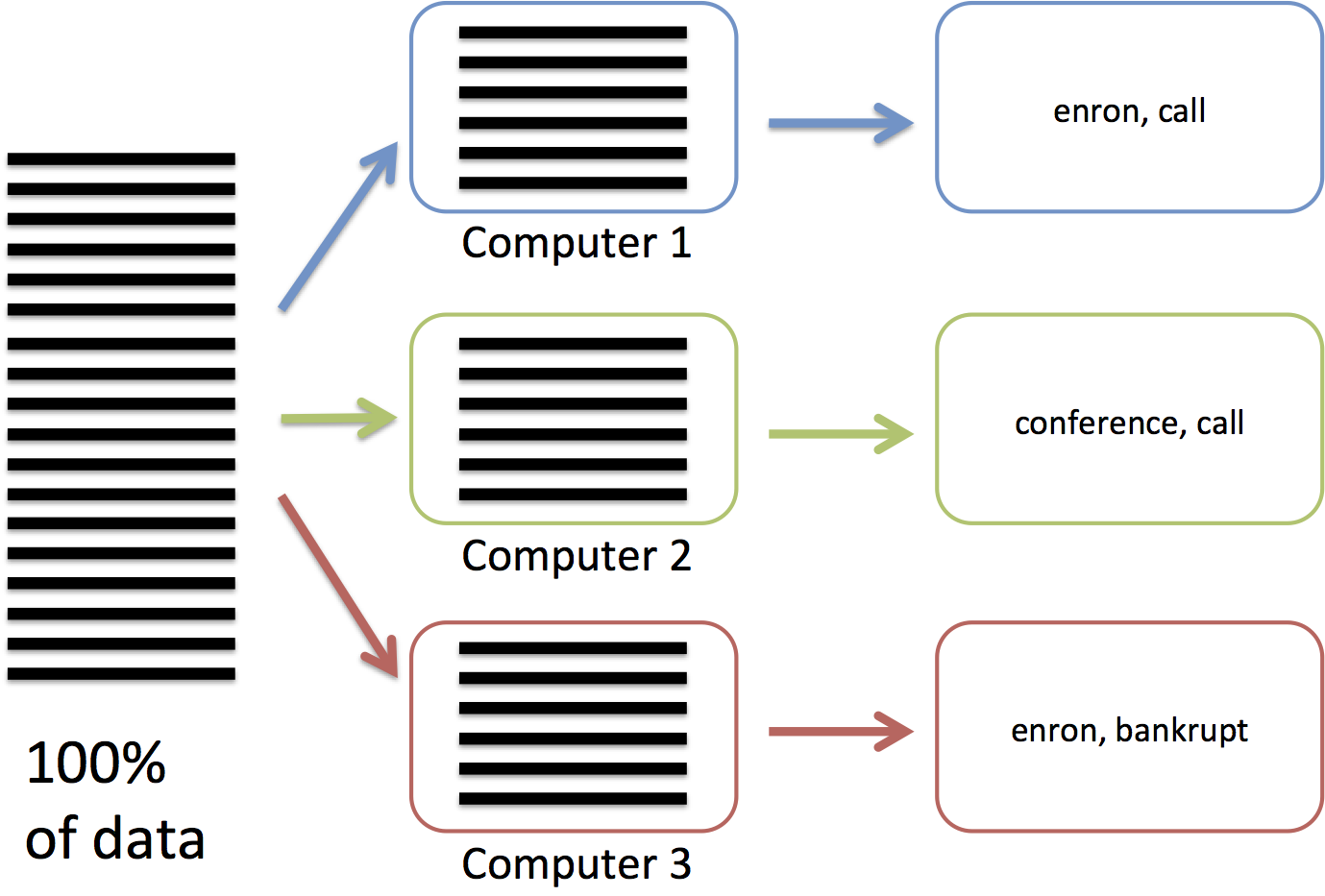
In the map phase (figure below), we are going to send each computer 1/3 of the lines. Each computer will process their 1,000,000 lines by reading each of the lines and tokenizing their words. For example, the first machine may extract "enron, call,...", while the second machine extracts "conference, call,...".

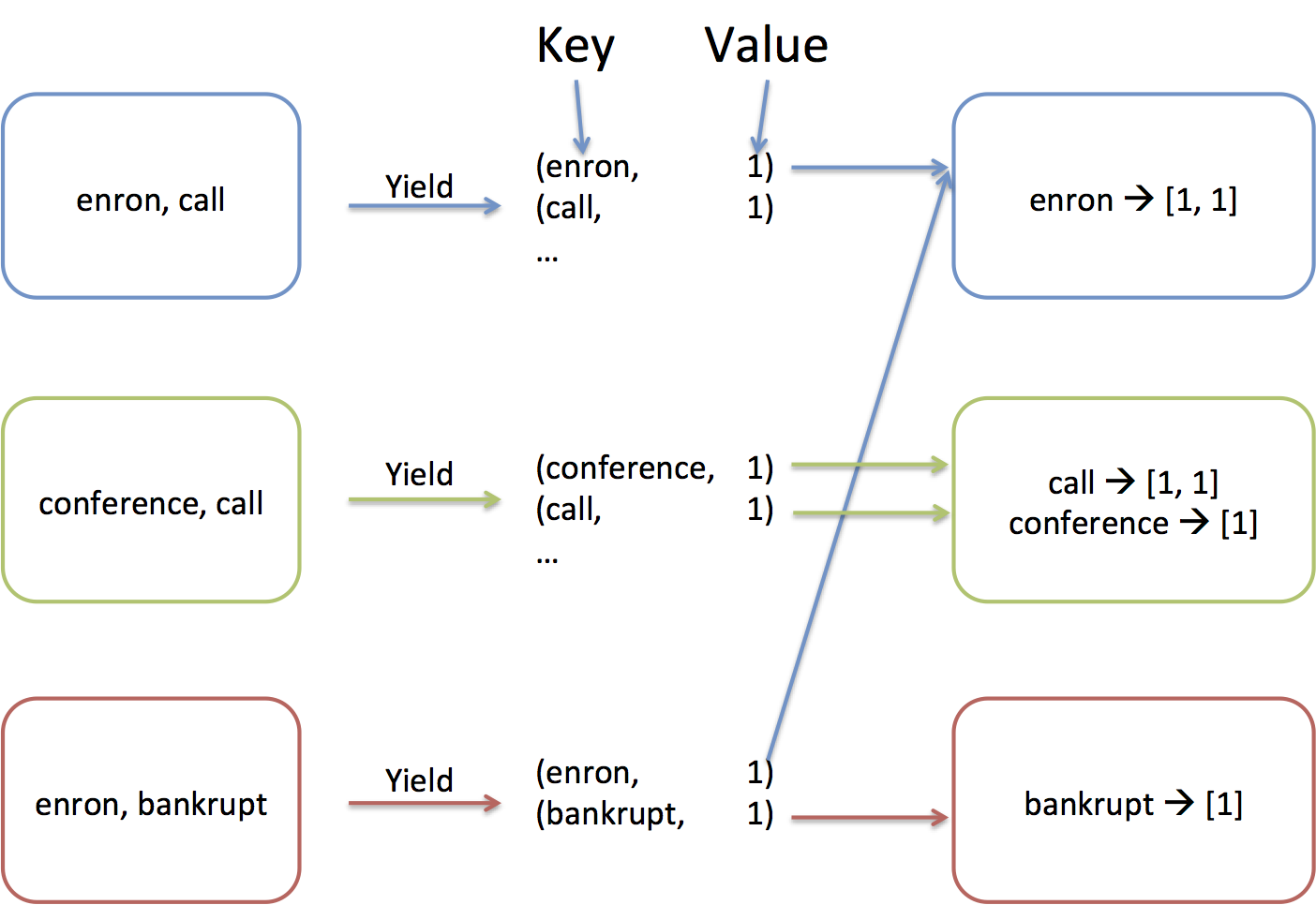
From the words, we will create (key, value) pairs (or (word, 1) pairs in this example). The shuffle phase will assigned each key to one of the 3 computer, and all the values associated with the same key are sent to the key's computer. This is necessary because the whole dictionary doesn't fit in the memory of a single computer! Think of this as creating the (key, value) pairs of a huge dictionary that spans all of the 3,000,000 emails. Because the whole dictionary doesn't fit into a single machine, the keys are distributed across our 3 machines. In this example, "enron" is assigned to computer 1, while "call" and "conference" are assigned to computer 2, and "bankrupt" is assigned to computer 3.

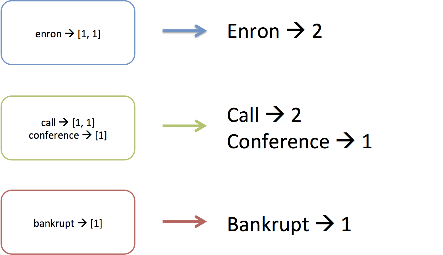
Finally, once each machine has received the values of the keys it's responsible for, the reduce phase will process each key's value. It does this by going through each key that is assigned to the machine and executing a reducer function on the values associated with the key. For example, "enron" was associated with a list of three 1's, and the reducer step simply adds them up.

MapReduce is more general-purpose than just serving to count words. Some people have used it to do exotic things like process millions of songs, but we want you to work through an entire end-to-end example.

Without further ado, here's the wordcount example, but written as a MapReduce application:

import sys
from mrjob.protocol import JSONValueProtocol
from mrjob.job import MRJob
from term_tools import get_terms

class MRWordCount(MRJob):
    INPUT_PROTOCOL = JSONValueProtocol
    OUTPUT_PROTOCOL = JSONValueProtocol

    def mapper(self, key, email):
        for term in get_terms(email['text']):
            yield term, 1

    def reducer(self, term, occurrences):
        yield None, {'term': term, 'count': sum(occurrences)}

if __name__ == '__main__':
        MRWordCount.run()
#

Let's break this thing down. You'll notice the term MRJob in a bunch of places. MRJob is a python package that makes writing MapReduce programs easy. The developers at Yelp (they wrote the mrjob module) wrote a convenience class called MRJob that you will extend. When it's run, it automatically hooks into the MapReduce framework, reads and parses the input files, and does a bunch of other things for you.

What we do is create a class MRWordCount that extends MRJob, and implement the mapper and reducer functions. If the program is run from the command line (the if __name__ == '__main__': part), it will execute the MRWordCount MapRedce program.

Looking inside MRWordCount, we see INPUT_PROTOCOL being set to JSONValueProtocol. By default, map functions expect a line of text as input, but we've encoded our emails as JSON, so we let MRJob know that. Similarly, we explain that our reduce tasks will emit dictionaries by setting OUTPUT_PROTOCOL appropriately.

The mapper function handles the functionality described in the first image of the last section. It takes each email, tokenizes it into terms, and yields each term. You can yield a key and a value (term and 1) in a mapper (notice "yield" arrows in the second figure above). We yield the term with the value 1, meaning one instance of the word term was found. yield is a python keyword that turns functions into iterators (stack overflow explanation). In the context of writing mapper and reducer functions, you can think of it as return.

The reducer function implements the third image of the last section. We are given a word (the key emitted from mappers), and a list occurrences of all of the values emitted for each instance of term. Since we are counting occurrences of words, we yield a dictionary containing the term and a sum of the occurrences we've seen.

Note that we sum instead of len the occurrences. This allows us to change the mapper implementation to emit the number of times each word occurs in a document, rather than 1 for each word.

Both the mapper and reducer offer us the parallelism we wanted. There is no loop through our entire set of emails, so MapReduce is free to distribute the emails to multiple machines, each of which will run mapper on an email-by-email basis. We don't have a single dictionary with the count of every word, but instead have a reduce function that has to sum up the occurrences of a single word, meaning we can again distribute the work to several reducing machines.

Run It!

Enough talk! Let's run this thing.

python mr_wordcount.py -o 'wordcount_test' --no-output '../datasets/emails/lay-k.json'
#

The -o flag tells MRJob to output all reducer output to the wordcount_test directory. The --no-output flag says not to print the output of the reducers to the screen. The last argument ('../datasets/emails/lay-k.json') specifies which file (or files) to read into the mappers as input.

Take a look at the newly created wordcount_test directory. There should be at least one file (part-00000), and perhaps more. There is one file per reducer that counted words. Reducers don't talk to one-another as they do their work, and so we end up with multiple output files. While the count of a specific word will only appear in one file, we have no idea which reducer file will contain a given word.

The output files (open one up in a text editor) list each word as a dictionary on a single line (OUTPUT_PROTOCOL = JSONValueProtocol in mr_wordcount.py is what caused this).

You will notice we have not yet run tasks on large datasets (we're still using lay-k.json) and we are still running them locally on our computers. We will soon learn to movet his work to Amazon's cloud infrastructure, but running MRJob tasks locally to test them on a small file is forever important. MapReduce tasks will take a long time to run and hold up several tens to several hundreds of machines. They also cost money to run, whether they contain a bug or not. Test them locally like we just did to make sure you don't have bugs before going to the full dataset.

Show off What you Learned

#

Exercise Create a second version of the MapReduce wordcounter that counts the number of each word emitted by each sender. You will need this for later, since we're going to be calculating TF-IDF implementing terms per sender. You can accomplish this with a sneaky change to the term emitted by the mapper. You can either turn that term into a dictionary, or into a more complicated string, but either way you will have to encode both sender and term information in that term. If you get stuck, take a peak at dataiap/day5/mr_wc_by_sender.py.

#

(Optional) Exercise The grep command on UNIX-like systems allows you to search text files for some term or terms. Typing grep hotdogs file1 will return all instances of the word hotdogs in the file file1. Implement a grep for emails. When a user uses your mapreduce program to find a word in the email collection, they will be given a list of the subjects and senders of all emails that contain the word. You might find you do not need a particularly smart reducer in this case: that's fine. If you're pressed for time, you can skip this exercise.

#

We now know how to write some pretty gnarly MapReduce programs, but they all run on our laptops. Sort of boring. It's time to move to the world of distributed computing, Amazon-style!

Amazon Web Services

Amazon Web Services (AWS) is Amazon's gift to people who don't own datacenters. It allows you to elastically request computation and storage resources at varied scales using different services. As a testiment to the flexibility of the services, companies like NetFlix are moving their entire operation into AWS.

In order to work with AWS, you will need to set up an account. If you're in the class, we will have given you a username, password, access key, and access secret. To use these accounts, you will have to login through a special class-only webpage. The same instructions work for people who are trying this at home, only you need to log in at the main AWS website.

The username and password log you into the AWS console so that you can click around its interface. In order to let your computer identify itself with AWS, you have to tell your computer your access key and secret. On UNIX-like platforms (GNU/Linux, BSD, MacOS), type the following:

export AWS_ACCESS_KEY_ID='your_key_id'
export AWS_SECRET_ACCESS_KEY='your_access_id'
#

On windows machines, type the following at the command line:

set AWS_ACCESS_KEY_ID=your_key_id
set AWS_SECRET_ACCESS_KEY=your_access_id
#

Replace your_key_id and your_access_id with the ones you were assigned.

That's it! There are more than a day's worth of AWS services to discuss, so let's stick with two of them: Simple Storage Service (S3) and Elastic MapReduce (EMR).

AWS S3

S3 allows you to store gigabytes, terabytes, and, if you'd like, petabytes of data in Amazon's datacenters. This is useful, because laptops often don't crunch and store more than a few hundred gigabytes worth of data, and storing it in the datacenter allows you to securely have access to the data in case of hardware failures. It's also nice because Amazon tries harder than you to have the data be always accessible.

In exchange for nice guarantees about scale and accessibility of data, Amazon charges you rent on the order of 14 cents per gigabyte stored per month.

Services that work on AWS, like EMR, read data from and store data to S3. When we run our MapReduce programs on EMR, we're going to read the email data from S3, and write word count data to S3.

S3 data is stored in buckets . Within a bucket you create, you can store as many files or folders as you'd like. The name of your bucket has to be unique across all of the people that store their stuff in S3. Want to make your own bucket? Let's do this!

This gives you a bucket, but the bucket has nothing in it! Poor bucket. Let's upload Kenneth Lay's emails.

Awesome! We just uploaded our first file to S3. Amazon is now hosting the file. We can access it over the web, which means we can share it with other researchers or process it in Elastic MapReduce. To save time, we've uploaded the entire enron dataset to https://dataiap-enron-json.s3.amazonaws.com/. Head over there to see all of the different Enron employee's files listed (the first three should be allen-p.json, arnold-j.json, and arora-h.json).

Two notes from here. First, uploading the file to S3 was just an exercise---we'll use the dataiap-enron-json bucket for our future exercises. That's because the total file upload is around 1.3 gigs, and we didn't want to put everyone through the pain of uploading it themselves. Second, most programmers don't use the web interface to upload their files. They instead opt to upload the files from the command line. If you have some free time, feel free to check out dataiap/resources/s3_util.py for a script that copies directories to and downloads buckets from S3.

Let's crunch through these files!

AWS EMR

We're about to process the entire enron dataset. Let's do a quick sanity check that our mapreduce wordcount script still works. We're about to get into the territory of spending money on the order of 10 cents per machine-hour, so we want to make sure we don't run into preventable problems that waste money.

python mr_wordcount.py -o 'wordcount_test2' --no-output '../datasets/emails/lay-k.json'
#

Did that finish running and output the word counts to wordcount_test2? If so, let's run it on 20 machines (costing us $2, rounded to the nearest hour). Before running the script, we'll talk about the parameters:

python mr_wordcount.py  --num-ec2-instances=20 --python-archive package.tar.gz -r emr -o 's3://dataiap-YOURUSERNAME-testbucket/output' --no-output 's3://dataiap-enron-json/*.json'
#

The parameters are:

Check back on the script. Is it still running? It should be. You may as well keep reading, since you'll be here a while. In total, our run took three minutes for Amazon to requisition the machines, four minutes to install the necessary software on them, and between 15 adn 25 minutes to run the actual MapReduce tasks on Hadoop. That might strike some of you as weird, and we'll talk about it now.

Understanding MapReduce is about understanding scale . We're used to thinking of our programs as being about performance , but that's not the role of MapReduce. Running a script on a single file on a single machine will be faster than running a script on multiple files split amongst multiple machines that shuffle data around to one-another and emit the data to a service (like EMR and S3) over the internet is not going to be fast. We write MapReduce programs because they let us easily ask for 10 times more machines when the data we're processing grows by a factor of 10, not so that we can achieve sub-second processing times on large datasets. It's a mental model switch that will take a while to appreciate, so let it brew in your mind for a bit.

What it does mean is that MapReduce as a programming model is not a magic bullet. The Enron dataset is not actually so large that it shouldn't be processed on your laptop. We used the dataset because it was large enough to give you an appreciation for order-of-magnitue file size differences, but not large enough that a modern laptop can't process the data. In practice, don't look into MapReduce until you have several tens or hundreds of gigabytes of data to analyze. In the world that exists inside most companies, this size dataset is easy to stumble upon. So don't be disheartened if you don't need the MapReduce skills just yet: you will likely need them one day.

Analyzing the output

Hopefully your first mapreduce is done by now. There are two bits of output we should check out. First, when the MapReduce job finishes, you will see something like the following message in your terminal window:

Counters from step 1:
  FileSystemCounters:
    FILE_BYTES_READ: 499365431
    FILE_BYTES_WRITTEN: 61336628
    S3_BYTES_READ: 1405888038
    S3_BYTES_WRITTEN: 8354556
  Job Counters :
    Launched map tasks: 189
    Launched reduce tasks: 85
    Rack-local map tasks: 189
  Map-Reduce Framework:
    Combine input records: 0
    Combine output records: 0
    Map input bytes: 1405888038
    Map input records: 516893
    Map output bytes: 585440070
    Map output records: 49931418
    Reduce input groups: 232743
    Reduce input records: 49931418
    Reduce output records: 232743
    Reduce shuffle bytes: 27939562
    Spilled Records: 134445547
#

That's a summary of, on your 20 machines, how many Mappers and Reducers ran. You can run more than one of each on a physical machine, which explains why more than 20 of each ran in our tasks. Notice how many reducers ran your task. Each reducer is going to receive a set of words and their number of occurrences, and emit word counts. Reducers don't talk to one-another, so they end up writing their own files.

With this in mind, go to the S3 console, and look at the output directory of the S3 bucket to which you output your words. Notice that there are several files in the output directory named part-00000, part-00001. There should be as many files as there were reducers, since each wrote the file out. Download some of these files and open them up. You will see the various word counts for words across the entire Enron email corpus. Life is good!

#

(Optional) Exercise : Make a directory called copied. Copy the output from your script to copied using dataiap/resources/s3_util.py with a command like python ../resources/s3_util get s3://dataiap-YOURUSERNAME-testbucket/output copied. Once you've got all the files downloaded, load them up and sort the lines by their count. Do the popular terms across the entire dataset make sense?

#

TF-IDF

This section is going to further exercise our MapReduce-fu.

On day 4, we learned that counting words is not enough to summarize text: common words like the and and are too popular. In order to discount those words, we multiplied by the term frequency of wordX by log(total # documents/# documents with wordX). Let's do that with MapReduce!

We're going to emit a per-sender TF-IDF. To do this, we need three MapReduce tasks:

HINT Do not run these MapReduce tasks on Amazon. You saw how slow it was to run, so make sure the entire TF-IDF workflow works on your local machine with lay-k.json before moving to Amazon.

MapReduce 1: Total Number of Documents

Eugene and I are the laziest of instructors. We don't like doing work where we don't have to. If you'd like a mental exercise as to how to write this MapReduce, you can do so yourself, but it's simpler than the wordcount example. Our dataset is small enough that we can just use the wc UNIX command to count the number of lines in our corpus:

wc -l lay-k.json
#

Kenneth Lay has 5929 emails in his dataset. We ran wc -l on the entire Enron email dataset, and got 516893. This took a few seconds. Sometimes, it's not worth overengineering a simple task!:)

MapReduce 2: Per-Term IDF

We recommend you stick to 516893 as your total number of documents, since eventually we're going to be crunching the entire dataset!

What we want to do here is emit log(516893.0 / # documents with wordX) for each wordX in our dataset. Notice the decimal on 516893.0: that's so we do floating point division rather than integer division. The output should be a file where each line contains {'term': 'wordX', 'idf': 35.92} for actual values of wordX and 35.92.

We've put our answer in dataiap/day5/mr_per_term_idf.py, but try your hand at writing it yourself before you look at ours. It can be implemented with a three-line change to the original wordcount MapReduce we wrote (one line just includes math.log!).

MapReduce 3: Per-Sender TF-IDFs

The third MapReduce multiplies per-sender term frequencies by per-term IDFs. This means it needs to take as input the IDFs calculated in the last step and calculate the per-sender TFs. That requires something we haven't seen yet: initialization logic. Let's show you the code, then tell you how it's done.

import os
from mrjob.protocol import JSONValueProtocol
from mrjob.job import MRJob
from term_tools import get_terms

DIRECTORY = "/path/to/idf_parts/"

class MRTFIDFBySender(MRJob):
    INPUT_PROTOCOL = JSONValueProtocol
    OUTPUT_PROTOCOL = JSONValueProtocol

    def mapper(self, key, email):
        for term in get_terms(email['text']):
            yield {'term': term, 'sender': email['sender']}, 1

    def reducer_init(self):
        self.idfs = {}
        for fname in os.listdir(DIRECTORY): # look through file names in the directory
            file = open(os.path.join(DIRECTORY, fname)) # open a file
            for line in file: # read each line in json file
                term_idf = JSONValueProtocol.read(line)[1] # parse the line as a JSON object
                self.idfs[term_idf['term']] = term_idf['idf']

    def reducer(self, term_sender, howmany):
        tfidf = sum(howmany) * self.idfs[term_sender['term']]
        yield None, {'term_sender': term_sender, 'tfidf': tfidf}
    
#

If you did the first exercise , the mapper and reducer functions should look a lot like the per-sender word count mapper and reducer functions you wrote for that. The only difference is that reducer takes the term frequencies and multiplies them by self.idfs[term], to normalize by each word's IDF. The other difference is the addition of reducer_init, which we will describe next.

self.idfs is a dictionary containing term-IDF mappings from the second MapReduce. Say you ran the IDF-calculating MapReduce like so:

python mr_per_term_idf.py -o 'idf_parts' --no-output '../datasets/emails/lay-k.json'
#

The individual terms and IDFs would be emitted to the directory idf_parts/. We would want to load all of these term-idf mappings into self.idfs. Set DIRECTORY to the filesystem path that points to the idf_parts/ directory.

Sometimes, we want to load some data before running the mapper or the reducer. In our example, we want to load the IDF values into memory before executing the reducer, so that the values are available when we compute the tf-idf. The function reducer_init is designed to perform this setup. It is called before the first reducer is called to calculate TF-IDF. It opens all of the output files in DIRECTORY, and reads them into self.idfs. This way, when reducer is called on a term, the idf for that term has already been calculated.

To verify you've done this correctly, compare your output to ours. There were some pottymouths that emailed Kenneth Lay:

{"tfidf": 13.155591168821202, "term_sender": {"term": "a-hole", "sender": "justinsitzman@hotmail.com"}}

Why is it OK to Load IDFs Into Memory?

You might be alarmed at the moment. Here we are, working with BIG DATA, and now we're expecting the TF-IDF calculation to load the entirety of the IDF data into memory on EVERY SINGLE reducer. That's crazytown.

It's actually not. While the corpus we're analyzing is large, the number of words in the English language (roughly the amount of terms we calculate IDF for) is not. In fact, the output of the per-term IDF calculation was around 8 megabytes, which is far smaller than the 1.3 gigabytes we processed. Keep this in mind: even if calculating something over a large amount of data is hard and takes a while, the result might end up small.

Optional: Run The TF-IDF Workflow

We recommend running the TF-IDF workflow on Amazon once class is over. The first MapReduce script (per-term IDF) should run just fine on Amazon. The second will not. The reducer_init logic expects a file to live on your local directory. You will have to modify it to read the output of the IDF calculations from S3 using boto. Take a look at the code to implement get in dataiap/resources/s3_util.py for a programmatic view of accessing files in S3.

Where to go from here

We hope that MapReduce serves you well with large datasets. If this kind of work excites you, here are some things to read up on.